
Working with Rows and Columns, Freezing Panes
There is also a video teaching you how to freeze a portion of the worksheet, for easy and effective scrolling.
The spreadsheet is a huge table, consisting of numerous rows and columns, which can be easily manipulated.
You can add or delete rows and columns, one by one, or many simultaneously.
The columns width, as well as the rows height can be adjusted carefully, to fit best your data.
Freezing panes comes to aid you when you scroll a big table, and the headers (titles) row and column have gone outside of the screen, making the table's data incomprehensible. Freezing them on the screen will keep them visible despite the scrolling.
Read here about the number of rows in the worksheet: Excel Row Limit
How to freeze panes (freezing rows and columns)
Let's assume we have the following worksheet: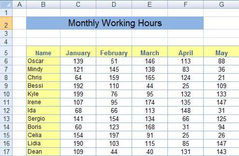
We wish to freeze the yellow rows and columns, so let's follow these steps:
1. Locate the meeting corner (the intersection) of the heading row and the heading column (in the above example: cell B5).
2. Select the cell that is in the inner part of that corner by clicking it (in our example: cell C6).
3. Choose the “View” tab from the ribbon.
4. Click the “Freeze Panes” button, and choose the first option (“Freeze Panes”).
Now you can scroll the window freely, the heading rows and columns will stay.
If you wish to cancel this, get back to the “Freeze Panes” button, and you can now choose “Unfreeze Panes”.
When should you freeze panes?
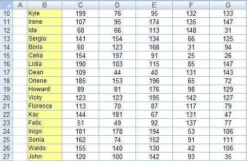
Let's assume that we scroll downwards the table given above.The moment the header row went out of the screen, we have lost the month indicators, and we are barely able to know what column relates to what month:
The problem gets worse when scrolling to the right, as can be seen here:
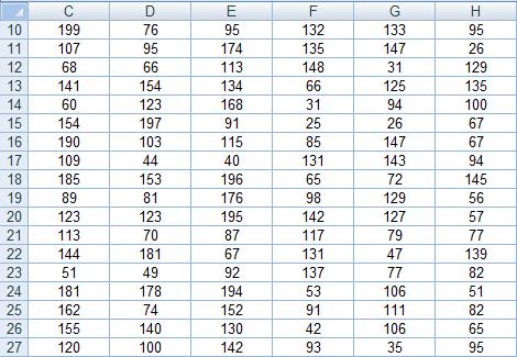
The table has no meaning now, just a stack of numbers.
The solution is to freeze the header rows and columns, so no matter how you scroll it, they remain on the screen, allowing you to relate the numbers to the corresponding months and employees, as can be seen in the following image:
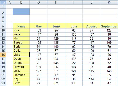
You can see that although rows 6-9 are missing, and columns C-F are missing due to the scrolling, the header row (5) and header column (B) are still visible, enabling us to relate the numerical data to its corresponding month and employee.